【3】数据分析-4-1-由煮面条到图论到图论--NetworkX

February 08, 2017 py_module 阅读量：次

今晚跟室友煮了个面条，满满的一锅面条，煮了好久，可是那些缠在一块的面条中间的那部分怎么都煮不熟，着实令人着急。一边煮面条，我就在想这一锅面条不正是一大堆引物放在一个管子里面做Multiplex PCR吗？有的引物可以放在一起煮，有的不能放在一起。那怎样可以满足尽可能减少试管，同时又能满足均一化呢？

一、NetworkX概论

NetworkX是一个用Python语言开发的图论与复杂网络建模工具，内置了常用的图与复杂网络分析算法，可以方便的进行复杂网络数据分析、仿真建模等工作。networkx支持创建简单无向图、有向图和多重图（multigraph）；内置许多标准的图论算法，节点可为任意数据；支持任意的边值维度，功能丰富，简单易用。

官网：http://networkx.github.io/index.html

官网教学：http://networkx.readthedocs.io/en/networkx-1.11/tutorial/

安装

pip install networkx

引入模块

import networkx as nx
print nx

无向图

例1：

#!-*- coding:utf8-*-
import networkx as nx
#linux系统下没有作图系统，需要如下生成图片
import matplotlib
matplotlib.use('Agg')
import matplotlib.pyplot as plt
#windows下直接
import matplotlib.pyplot as plt
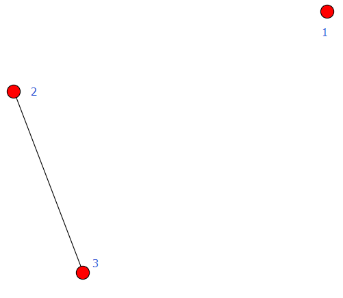
G = nx.Graph() #建立一个空的无向图G G.add_node(1) #添加一个节点1 
G.add_edge(2,3) #添加一条边2-3（隐含着添加了两个节点2、3） 
G.add_edge(3,2) #对于无向图，边3-2与边2-3被认为是一条边 
print "nodes:", G.nodes() #输出全部的节点： [1, 2, 3] 
print "edges:", G.edges() #输出全部的边：[(2, 3)] 
print "number of edges:", G.number_of_edges() #输出边的数量：1 
nx.draw(G,with_labels=True) #nodes的标签加上
plt.savefig("wuxiangtu.png") 
plt.show()

输出：

nodes: [1, 2, 3]
edges: [(2, 3)]
number of edges: 1

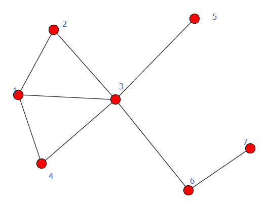
例2：

#-*- coding:utf8-*-
 
import networkx as nx
import matplotlib.pyplot as plt
G = nx.DiGraph()
G.add_node(1)
G.add_node(2)                  #加点
G.add_nodes_from([3,4,5,6])    #加点集合
G.add_cycle([1,2,3,4])         #加环
G.add_edge(1,3)     
G.add_edges_from([(3,5),(3,6),(6,7)])  #加边集合
nx.draw(G)
plt.savefig("youxiangtu.png")
plt.show()

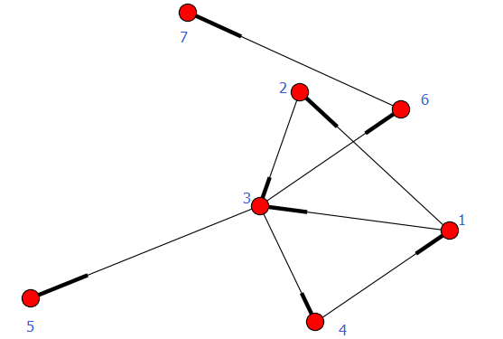
有向图

例1：

#!-*- coding:utf8-*-
 
import networkx as nx
import matplotlib.pyplot as plt

G = nx.DiGraph()
G.add_node(1)
G.add_node(2)
G.add_nodes_from([3,4,5,6])
G.add_cycle([1,2,3,4])
G.add_edge(1,3)
G.add_edges_from([(3,5),(3,6),(6,7)])
nx.draw(G)
plt.savefig("youxiangtu.png")
plt.show()

注：有向图和无向图可以互相转换，使用函数：

Graph.to_undirected()
Graph.to_directed()

例2，例子中把有向图转化为无向图：

#!-*- coding:utf8-*-
 
import networkx as nx
import matplotlib.pyplot as plt

G = nx.DiGraph()
G.add_node(1)
G.add_node(2)
G.add_nodes_from([3,4,5,6])
G.add_cycle([1,2,3,4])
G.add_edge(1,3)
G.add_edges_from([(3,5),(3,6),(6,7)])
G = G.to_undirected()
nx.draw(G)
plt.savefig("wuxiangtu.png")
plt.show()

注意区分以下2例

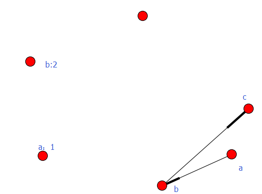
例3-1

#-*- coding:utf8-*-

import networkx as nx
import matplotlib.pyplot as plt

G = nx.DiGraph()

road_nodes = {'a': 1, 'b': 2, 'c': 3}
#road_nodes = {'a':{1:1}, 'b':{2:2}, 'c':{3:3}}
road_edges = [('a', 'b'), ('b', 'c')]

G.add_nodes_from(road_nodes.iteritems())
G.add_edges_from(road_edges)

nx.draw(G)
plt.savefig("youxiangtu.png")
plt.show()

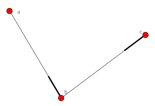
例3-2

#-*- coding:utf8-*-

import networkx as nx
import matplotlib.pyplot as plt

G = nx.DiGraph()

#road_nodes = {'a': 1, 'b': 2, 'c': 3}
road_nodes = {'a':{1:1}, 'b':{2:2}, 'c':{3:3}}
road_edges = [('a', 'b'), ('b', 'c')]

G.add_nodes_from(road_nodes.iteritems())
G.add_edges_from(road_edges)

nx.draw(G)
plt.savefig("youxiangtu.png")
plt.show()

加权图

有向图和无向图都可以给边赋予权重，用到的方法是add_weighted_edges_from，它接受1个或多个三元组[u,v,w]作为参数，其中u是起点，v是终点，w是权重。

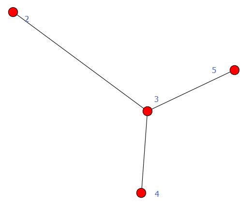
例1：

import networkx as nx
import matplotlib.pyplot as plt
G = nx.Graph()                                        #建立一个空的无向图G
G.add_edge(2,3)                                     #添加一条边2-3（隐含着添加了两个节点2、3）
G.add_weighted_edges_from([(3, 4, 3.5),(3, 5, 7.0)])                                     #对于无向图，边3-2与边2-3被认为是一条边
	
print G.get_edge_data(2, 3)
print G.get_edge_data(3, 4)
print G.get_edge_data(3, 5)

nx.draw(G)
plt.savefig("wuxiangtu.png")
plt.show()

输出

{}
{'weight': 3.5}
{'weight': 7.0}

经典图论算法计算

计算1：求无向图的任意两点间的最短路径

import networkx as nx
import matplotlib.pyplot as plt
 
#计算1：求无向图的任意两点间的最短路径
G = nx.Graph()
G.add_edges_from([(1,2),(1,3),(1,4),(1,5),(4,5),(4,6),(5,6)])
path = nx.all_pairs_shortest_path(G)
print path[1]

强连通、弱连通

强连通：有向图中任意两点v1、v2间存在v1到v2的路径（path）及v2到v1的路径。
弱联通：将有向图的所有的有向边替换为无向边，所得到的图称为原图的基图。如果一个有向图的基图是连通图，则有向图是弱连通图。

例1：弱连通

import networkx as nx
import matplotlib.pyplot as plt
#G = nx.path_graph(4, create_using=nx.Graph())
#0 1 2 3
G = nx.path_graph(4, create_using=nx.DiGraph())    #默认生成节点0 1 2 3，生成有向变0->1,1->2,2->3
G.add_path([7, 8, 3])  #生成有向边：7->8->3

for c in nx.weakly_connected_components(G):
	print c

print [len(c) for c in sorted(nx.weakly_connected_components(G), key=len, reverse=True)]

nx.draw(G)
plt.savefig("youxiangtu.png")
plt.show()

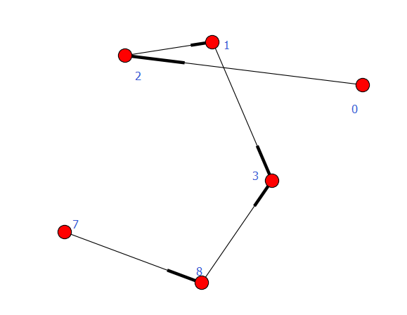
执行结果

set([0, 1, 2, 3, 7, 8])
[6]

例2：强连通

import networkx as nx
import matplotlib.pyplot as plt
#G = nx.path_graph(4, create_using=nx.Graph())
#0 1 2 3
G = nx.path_graph(4, create_using=nx.DiGraph())
G.add_path([3, 8, 1])

#for c in nx.strongly_connected_components(G):
#    print c
#
#print [len(c) for c in sorted(nx.strongly_connected_components(G), key=len, reverse=True)]	

con = nx.strongly_connected_components(G)
print con
print type(con)
print list(con)

nx.draw(G)
plt.savefig("youxiangtu.png")
plt.show()

执行结果

<type 'generator'>
[set([8, 1, 2, 3]), set([0])]

子图

import networkx as nx
import matplotlib.pyplot as plt
G = nx.DiGraph()
G.add_path([5, 6, 7, 8])
sub_graph = G.subgraph([5, 6, 8])
#sub_graph = G.subgraph((5, 6, 8))  #ok  一样

nx.draw(sub_graph)
plt.savefig("youxiangtu.png")
plt.show()

二、其他函数

planted_partition_graph

planted_partition_graph(l, k, p_in, p_out, seed=None, directed=False)

函数详解：

Return the planted l-partition graph.

This model partitions a graph with n=l*k vertices in l groups with k vertices each. Vertices of the same group are linked with a probability p_in, and vertices of different groups are linked with probability p_out.

Parameters:	
l (int) – Number of groups
k (int) – Number of vertices in each group
p_in (float) – probability of connecting vertices within a group
p_out (float) – probability of connected vertices between groups
seed (int,optional) – Seed for random number generator(default=None)
directed (bool,optional (default=False)) – If True return a directed graph
Returns:	
G – planted l-partition graph

Return type:	
NetworkX Graph or DiGraph

Raises:	
NetworkXError: – If p_in,p_out are not in [0,1] or

具体例子

import networkx as nx
gene_net = nx.planted_partition_graph(50, 10, 0.2, 0.05, seed=42)  # 50组，每10个，算是500个了吧

## 理解这是什么图

# ## 1.把图做出来
# nx.draw(gene_net)
# plt.savefig('test.png')
# plt.show()

# 2.查看nodes
# print gene_net.nodes()
#看到了0-499 的list，说明应该是 500个nodes，难道是 50 *10 ？

# 3.输出图的边值
# print gene_net.edges()
# 出来的是 0-499任意两个数的set。

# 其他属性

# print gene_net.degree()
# print gene_net.degree_histogram()
# print gene_net.density()

# print nx.info(gene_net)
# Type: Graph
# Number of nodes: 500
# Number of edges: 6566
# Average degree:  26.2640

# print nx.is_directed(gene_net)
# False

## 获得Nodes
# print len(nx.nodes(gene_net))
# 500

2.2 独立的node，即没有Node与其形成edge

import networkx as nx
G = nx.path_graph(4)
G.add_edge(5,6)
G.add_node(7)
G.add_node(8)
graphs = list(nx.isolates(G))
for one_part in graphs:
    print(one_part)

结果：

7
8

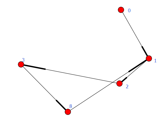
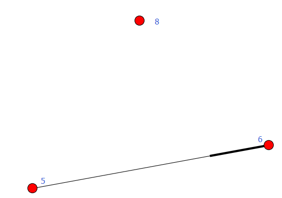
2.3 连通子图，子图里面不需要任意两两之间相连

import networkx as nx
G = nx.path_graph(4)
G.add_edge(5,6)
G.add_edge(5,7)
graphs = list(nx.connected_component_subgraphs(G))
for one_part in graphs:
    print(one_part.nodes)

结果：

[0, 1, 2, 3]
[5, 6, 7]

2.4 任意两点之间的联通

同时适用于有向图哦

G = nx.complete_graph(4)
for path in nx.all_simple_paths(G, source=0, target=3):
	print(path)

[0, 1, 2, 3]
[0, 1, 3]
[0, 2, 1, 3]
[0, 2, 3]
[0, 3]

paths = nx.all_simple_paths(G, source=0, target=3, cutoff=2)
print(list(paths))
[[0, 1, 3], [0, 2, 3], [0, 3]]

说明：

source :起点Node
target: 终点node
cutoff:  Depth to stop the search. Only paths of length <= cutoff are returned

2.5 最短path

G = nx.path_graph(5)
path = nx.all_pairs_shortest_path(G)

print(path[0][4])
[0, 1, 2, 3, 4]

2.6 最长path

不适用于环状的图

def longest_path(G):
    dist = {} # stores [node, distance] pair
    for node in nx.topological_sort(G):
        # pairs of dist,node for all incoming edges
        pairs = [(dist[v][0]+1,v) for v in G.pred[node]] 
        if pairs:
            dist[node] = max(pairs)
        else:
            dist[node] = (0, node)
    node,(length,_)  = max(dist.items(), key=lambda x:x[1])
    path = []
    while length > 0:
        path.append(node)
        length,node = dist[node]
    return list(reversed(path))

if __name__=='__main__':
    G = nx.DiGraph()
    G.add_path([1,2,3,4])
    G.add_path([1,20,30,31,32,4])
    nx.draw(G, with_labels=True,font_size=20)
    #    G.add_path([20,2,200,31])
    print(longest_path(G))

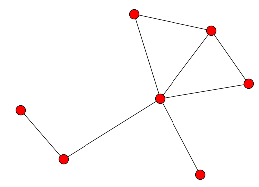
三、案例：

import networkx as nx
from networkx.algorithms.approximation.clique import max_clique, clique_removal

G = nx.Graph()
G.add_edge(primer1, primer2)
nx.draw(G, with_labels=True)
plt.savefig('temp/network.png')
plt.show()

各种有可能的连通图的组合
cliques_primers1 = list(nx.find_cliques(G))

找到最大的连通图，然后去除图中的东西，接着找下一个图
cliques_primers2 = list(list(clique_removal(G))[1])

四、讨论：

1.加颜色

import networkx as nx
import numpy as np
import matplotlib.pyplot as plt

G = nx.Graph()
G.add_edges_from(
	[('A', 'B'), ('A', 'C'), ('D', 'B'), ('E', 'C'), ('E', 'F'),
	 ('B', 'H'), ('B', 'G'), ('B', 'F'), ('C', 'G')])

val_map = {'A': 1.0,
		   'D': 0.5714285714285714,
		   'H': 0.0}

values = [val_map.get(node, 0.25) for node in G.nodes()]

nx.draw(G, cmap=plt.get_cmap('jet'), node_color=values)

# nx.draw(G, cmap=plt.get_cmap('viridis'), node_color=values, with_labels=True, font_color='white')  #其他颜色： PuBuGn , PuBuGn_r

plt.show()

参考资料

药企，独角兽，苏州。团队长期招人，感兴趣的都可以发邮件聊聊：tiehan@sina.cn

个人公众号，比较懒，很少更新，可以在上面提问题，如果回复不及时，可发邮件给我： tiehan@sina.cn